Introduction

Does drinking coffee actually increase your life expectancy? A recent study (Freedman, Park, Abnet, Hollenbeck, & Sinha, 2012) found that men who drank at least six cups of coffee a day had a 10% lower chance of dying (women 15% lower) than those who drank none. Does this mean you should pick up or increase your own coffee habit?

커피를 마시면 실제로 기대 수명이 늘어날까요? 최근의 한 연구(Freedman, Park, Abnet, Hollenbeck, & Sinha, 2012)에 따르면 하루에 커피를 6잔 이상 마시는 남성은 전혀 마시지 않는 사람보다 사망할 확률이 10%(여성은 15%) 낮았습니다. 그렇다면 커피를 마시는 습관을 만들거나 커피를 더 마셔야 할까요?

Modern society has become awash in studies such as this; you can read about several such studies in the news every day. Moreover, data abound everywhere in modern life. Conducting such a study well, and interpreting the results of such studies well for making informed decisions or setting policies, requires understanding basic ideas of statistics, the science of gaining insight from data. Rather than relying on anecdote and intuition, statistics allows us to systematically study phenomena of interest.

현대 사회는 이와 같은 연구로 넘쳐나고 있으며, 매일 뉴스에서 이러한 연구에 대한 소식을 접할 수 있습니다. 게다가 현대 생활의 모든 곳에 데이터가 넘쳐납니다. 이러한 연구를 잘 수행하고 그 결과를 잘 해석하여 정보에 입각한 의사 결정이나 정책 수립에 활용하려면 데이터에서 통찰을 얻는 과학인 통계의 기본 개념을 이해해야 합니다. 통계는 경험이나 직관에 의존하지 않고 관심 있는 현상을 체계적으로 연구할 수 있게 해줍니다.

통계 조사의 핵심 요소:

• Planning the study: Start by asking a testable research question and deciding how to collect data. For example, how long was the study period of the coffee study? How many people were recruited for the study, how were they recruited, and from where? How old were they? What other variables were recorded about the individuals, such as smoking habits, on the comprehensive lifestyle questionnaires? Were changes made to the participants’ coffee habits during the course of the study?
• 연구 계획 세우기: 실험 가능한 연구 질문을 던지고 데이터 수집 방법을 결정하는 것부터 시작하세요. 예를 들어, 커피 연구의 연구 기간은 얼마나 되었나요? 연구에 모집된 사람은 몇 명이며, 어디서 어떻게 모집했나요? 참가자의 나이는 몇 살이었나요? 종합적인 라이프스타일 설문지에 흡연 습관 등 개인에 대한 다른 어떤 변수가 기록되었나요? 연구가 진행되는 동안 참가자들의 커피 습관에 변화가 있었나요?
• Examining the data: What are appropriate ways to examine the data? What graphs are relevant, and what do they reveal? What descriptive statistics can be calculated to summarize relevant aspects of the data, and what do they reveal? What patterns do you see in the data? Are there any individual observations that deviate from the overall pattern, and what do they reveal? For example, in the coffee study, did the proportions differ when we compared the smokers to the non-smokers?
• 데이터 검토하기: 데이터를 검토하는 적절한 방법은 무엇인가요? 어떤 그래프가 관련성이 있으며, 무엇을 알려주는가? 데이터의 관련 측면을 요약하기 위해 계산할 수 있는 설명적 통계는 무엇이며, 이를 통해 알 수 있는 것은 무엇인가요? 데이터에서 어떤 패턴을 볼 수 있나요? 전체 패턴에서 벗어나는 개별적인 관찰 결과가 있으며, 이를 통해 무엇을 알 수 있나요? 예를 들어, 커피 연구에서 흡연자와 비흡연자를 비교했을 때 그 비율이 달랐나요?
• Inferring from the data: What are valid statistical methods for drawing inferences “beyond” the data you collected? In the coffee study, is the 10%–15% reduction in risk of death something that could have happened just by chance?
• 데이터에서 추론하기: 수집한 데이터를 '넘어서' 추론을 도출하는 데 유효한 통계적 방법은 무엇일까요? 커피 연구에서 사망 위험이 10~15% 감소한 것은 우연히 일어날 수 있는 일인가요?
• Drawing conclusions: Based on what you learned from your data, what conclusions can you draw? Who do you think these conclusions apply to? (Were the people in the coffee study older? Healthy? Living in cities?) Can you draw a cause-and-effect conclusion about your treatments? (Are scientists now saying that the coffee drinking is the cause of the decreased risk of death?)
• 결론 도출하기: 데이터에서 배운 내용을 바탕으로 어떤 결론을 도출할 수 있나요? 이러한 결론이 누구에게 적용될 수 있다고 생각하시나요? (커피 연구에 참여한 사람들은 나이가 많았나요? 건강했나요? 도시에 살았나요?) 치료에 대한 인과관계 결론을 도출할 수 있나요? (과학자들은 이제 커피를 마시는 것이 사망 위험 감소의 원인이라고 말하고 있나요?)

Notice that the numerical analysis (“crunching numbers” on the computer) comprises only a small part of overall statistical investigation. In this module, you will see how we can answer some of these questions and what questions you should be asking about any statistical investigation you read about.

수치 분석("컴퓨터에서 숫자를 계산하는 것")은 전체 통계 조사의 일부에 불과하다는 점에 유의하세요. 이 모듈에서는 이러한 질문에 답하는 방법과 읽은 통계 조사에 대해 어떤 질문을 해야 하는지 살펴봅니다.

분포적 사고(Distributional Thinking)

When data are collected to address a particular question, an important first step is to think of meaningful ways to organize and examine the data. The most fundamental principle of statistics is that data vary. The pattern of that variation is crucial to capture and to understand. Often, careful presentation of the data will address many of the research questions without requiring more sophisticated analyses. It may, however, point to additional questions that need to be examined in more detail.

특정 질문을 해결하기 위해 데이터를 수집할 때 중요한 첫 번째 단계는 데이터를 구성하고 조사하는 의미 있는 방법을 생각하는 것입니다. 통계의 가장 기본적인 원칙은 데이터는 변한다는 것입니다. 이러한 변화의 패턴을 포착하고 이해하는 것이 중요합니다. 데이터를 주의 깊게 표현하면 더 정교한 분석 없이도 많은 연구 질문을 해결할 수 있는 경우가 많습니다. 그러나, 더 자세히 조사해야 할 추가적인 질문으로 이끌 수 있습니다.

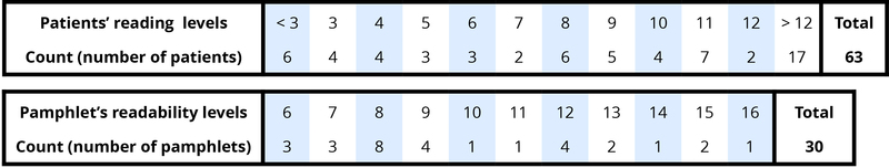
Example 1: Researchers investigated whether cancer pamphlets are written at an appropriate level to be read and understood by cancer patients (Short, Moriarty, & Cooley, 1995). Tests of reading ability were given to 63 patients. In addition, readability level was determined for a sample of 30 pamphlets, based on characteristics such as the lengths of words and sentences in the pamphlet. The results, reported in terms of grade levels, are displayed in Table 1.

예시 1: 연구자들은 암 팸플릿이 암 환자들이 읽고 이해하기에 적절한 수준으로 작성되었는지 조사했습니다(Short, Moriarty, & Cooley, 1995). 63명의 환자를 대상으로 읽기 능력 테스트를 실시했습니다. 또한 팜플렛의 단어 및 문장 길이와 같은 특성을 기준으로 30개의 팜플렛 샘플에 대한 가독성 수준을 측정했습니다. 학년별로 보고된 결과는 표 1에 나와 있습니다.

These two variables reveal two fundamental aspects of statistical thinking:

다음 두 변수는 통계학적 사고의 두 가지 근본적인 관점을 보여줍니다:

• Data vary. More specifically, values of a variable (such as reading level of a cancer patient or readability level of a cancer pamphlet) vary.
• Analyzing the pattern of variation, called the distribution of the variable, often reveals insights.

• 데이터는 변합니다. 더 정확하게는, 변수의 값(예: 암 환자의 독서 수준 또는 암 팸플릿의 가독성 수준) 은 변합니다.
• 변수의 분포라고 하는 변화의 패턴을 분석하면 종종 통찰을 얻을 수 있습니다. 

Addressing the research question of whether the cancer pamphlets are written at appropriate levels for the cancer patients requires comparing the two distributions. A naïve comparison might focus only on the centers of the distributions. Both medians turn out to be ninth grade, but considering only medians ignores the variability and the overall distributions of these data. A more illuminating approach is to compare the entire distributions, for example with a graph, as in Figure 1.

암 팸플릿이 암 환자에게 적절한 수준으로 작성되었는지에 대한 연구 문제를 해결하려면 두 가지 분포를 비교해야 합니다. 단순한 비교는 분포의 중앙에만 초점을 맞출지 모릅니다. 두 데이터의 중앙값은 모두 9학년으로 나타났지만 중앙값만 고려하면 데이터의 변동성과 전체 분포를 무시하게 됩니다. 그림 1에서와 같이 그래프를 사용하여 전체 분포를 비교하는 것이 더 나은 접근 방식입니다.

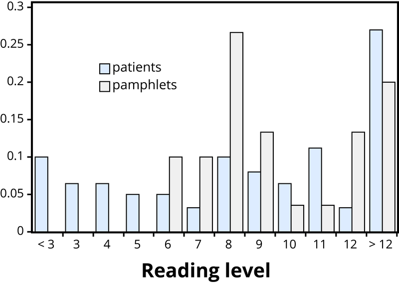
Figure 1 makes clear that the two distributions are not well aligned at all. The most glaring discrepancy is that many patients (17/63, or 27%, to be precise) have a reading level below that of the most readable pamphlet. These patients will need help to understand the information provided in the cancer pamphlets. Notice that this conclusion follows from considering the distributions as a whole, not simply measures of center or variability, and that the graph contrasts those distributions more immediately than the frequency tables.

그림 1을 보면 두 분포가 전혀 일치하지 않는다는 것을 알 수 있습니다. 가장 눈에 띄는 불일치는 많은 환자(17/63, 정확히 27%)가 가장 읽기 쉬운 팜플렛의 읽기 수준보다 낮다는 점입니다. 이러한 환자들은 암 팸플릿에 제공된 정보를 이해하는 데 도움이 필요합니다. 이러한 결론은 단순히 중심값이나 변동성을 측정하는 것이 아니라 전체 분포를 고려한 결과이며, 그래프가 빈도 표보다 더 즉각적으로 분포를 대조한다는 점에 유의하세요.

통계적 유의성

Even when we find patterns in data, often there is still uncertainty in various aspects of the data. For example, there may be potential for measurement errors (even your own body temperature can fluctuate by almost 1 °F over the course of the day). Or we may only have a “snapshot” of observations from a more long-term process or only a small subset of individuals from the population of interest. In such cases, how can we determine whether patterns we see in our small set of data is convincing evidence of a systematic phenomenon in the larger process or population?

데이터에서 패턴을 발견하더라도 데이터의 다양한 측면에는 여전히 불확실성이 존재하는 경우가 많습니다. 예를 들어, 측정 오류의 가능성이 있을 수 있습니다(심지어 자신의 체온도 하루 동안 거의 1°F까지 변동될 수 있습니다). 또는 장기적인 과정에서의 한 순간뿐의 데이터나 또는 관심 대상 집단에서 일부 개인만 관찰한 데이터만 있을 수도 있습니다. 이러한 경우, 작은 데이터 집합에서 보이는 패턴이 더 큰 프로세스 또는 집단에서 보이는 조직적인 현상에 대한 확실한 증거인지 어떻게 판단할 수 있을까요?

Example 2: In a study reported in the November 2007 issue of Nature, researchers investigated whether pre-verbal infants take into account an individual’s actions toward others in evaluating that individual as appealing or aversive (Hamlin, Wynn, & Bloom, 2007). In one component of the study, 10-month-old infants were shown a “climber” character (a piece of wood with “googly” eyes glued onto it) that could not make it up a hill in two tries. Then the infants were shown two scenarios for the climber’s next try, one where the climber was pushed to the top of the hill by another character (“helper”), and one where the climber was pushed back down the hill by another character (“hinderer”). The infant was alternately shown these two scenarios several times. Then the infant was presented with two pieces of wood (representing the helper and the hinderer characters) and asked to pick one to play with. The researchers found that of the 16 infants who made a clear choice, 14 chose to play with the helper toy.

예 2: 2007년 11월호 Nature에 보고된 한 연구에서 연구자들은 언어가 발달하기 전인 유아가 다른 사람을 평가할 때 그 사람이 매력적이거나 혐오스러운지 평가할 때 그 사람의 행동을 고려하는지 조사했습니다(Hamlin, Wynn, & Bloom, 2007). 연구의 한 구성 요소에서 10개월 된 유아에게 두 번의 시도에서 언덕을 오르지 못하는 "클라이머" 캐릭터(나무 조각에 플라스틱 눈알이 붙어 있는)를 보여주었습니다. 그런 다음 유아에게 등반가의 다음 시도에 대한 두 가지 시나리오를 보여주었습니다. 하나는 등반가가 다른 캐릭터("도우미")에 의해 언덕 꼭대기까지 밀려 올라가는 시나리오이고, 다른 캐릭터("방해자")에 의해 언덕 아래로 밀려 내려가는 시나리오입니다. 유아에게 이 두 가지 시나리오를 번갈아 가며 여러 번 보여주었습니다. 그런 다음 유아에게 두 개의 나무 조각(도우미와 방해꾼 캐릭터를 나타냄)을 제시하고 하나를 골라 가지고 놀도록 요청했습니다. 연구진은 명확한 선택을 한 16명의 유아 중 14명이 도우미 장난감을 가지고 놀기로 선택했다는 사실을 발견했습니다.

One possible explanation for this clear majority result is that the helping behavior of the one toy increases the infants’ likelihood of choosing that toy. But are there other possible explanations? What about the color of the toy? Well, prior to collecting the data, the researchers arranged so that each color and shape (red square and blue circle) would be seen by the same number of infants. Or maybe the infants had right-handed tendencies and so picked whichever toy was closer to their right hand? Well, prior to collecting the data, the researchers arranged it so half the infants saw the helper toy on the right and half on the left. Or, maybe the shapes of these wooden characters (square, triangle, circle) had an effect? Perhaps, but again, the researchers controlled for this by rotating which shape was the helper toy, the hinderer toy, and the climber. When designing experiments, it is important to control for as many variables as might affect the responses as possible.

이 명백한 결과에 대한 한 가지 가능한 설명은 한 장난감의 도움 행동이 유아가 그 장난감을 선택할 가능성을 높인다는 것입니다. 하지만 다른 가능한 설명이 있을까요? 장난감의 색깔은 어떨까요? 데이터를 수집하기 전에 연구진은 각 색상과 모양(빨간색 사각형과 파란색 원)을 같은 수의 유아가 볼 수 있도록 배치했습니다. 아니면 유아들이 오른손잡이 성향이 있어서 오른손에 더 가까운 장난감을 골랐을까요? 연구진은 데이터를 수집하기 전에 유아의 절반이 도우미 장난감을 오른쪽에서, 절반이 왼쪽에서 볼 수 있도록 배치했습니다. 아니면 나무 캐릭터의 모양(사각형, 삼각형, 원)이 영향을 미쳤을까요? 아마도 그럴 수도 있지만, 연구자들은 도우미 장난감, 방해 장난감, 클라이머 장난감의 모양을 바꿔서 실험을 진행하여 이를 통제했습니다. 실험을 설계할 때는 반응에 영향을 미칠 수 있는 변수를 최대한 많이 통제하는 것이 중요합니다.

It is beginning to appear that the researchers accounted for all the other plausible explanations. But there is one more important consideration that cannot be controlled—if we did the study again with these 16 infants, they might not make the same choices. In other words, there is some randomness inherent in their selection process. Maybe each infant had no genuine preference at all, and it was simply “random luck” that led to 14 infants picking the helper toy. Although this random component cannot be controlled, we can apply a probability model to investigate the pattern of results that would occur in the long run if random chance were the only factor.

연구자들이 다른 모든 그럴듯한 설명을 설명한 것으로 보이기 시작했습니다. 그러나 통제할 수 없는 한 가지 중요한 고려 사항이 더 있는데, 바로 16명의 유아를 대상으로 다시 연구를 진행한다면 동일한 선택을 하지 않을 수도 있다는 점입니다. 즉, 선택 과정에는 어느 정도 무작위성이 내재되어 있다는 것입니다. 어쩌면 각 유아는 진정한 선호도가 전혀 없었을 수도 있고, 14명의 유아가 도우미 장난감을 선택한 것은 단순히 "무작위적인 운"이었을 수도 있습니다. 이러한 무작위 요소는 통제할 수 없지만 확률 모델을 적용하여 무작위적 우연이 유일한 요인일 경우 장기적으로 발생할 수 있는 결과의 패턴을 조사할 수 있습니다.

If the infants were equally likely to pick between the two toys, then each infant had a 50% chance of picking the helper toy. It’s like each infant tossed a coin, and if it landed heads, the infant picked the helper toy. So if we tossed a coin 16 times, could it land heads 14 times? Sure, it’s possible, but it turns out to be very unlikely. Getting 14 (or more) heads in 16 tosses is about as likely as tossing a coin and getting 9 heads in a row. This probability is referred to as a p-value. The p-value tells you how often a random process would give a result at least as extreme as what was found in the actual study, assuming there was nothing other than random chance at play. So, if we assume that each infant was choosing equally, then the probability that 14 or more out of 16 infants would choose the helper toy is found to be 0.0021. We have only two logical possibilities: either the infants have a genuine preference for the helper toy, or the infants have no preference (50/50) and an outcome that would occur only 2 times in 1,000 iterations happened in this study. Because this p-value of 0.0021 is quite small, we conclude that the study provides very strong evidence that these infants have a genuine preference for the helper toy. We often compare the p-value to some cut-off value (called the level of significance, typically around 0.05). If the p-value is smaller than that cut-off value, then we reject the hypothesis that only random chance was at play here. In this case, these researchers would conclude that significantly more than half of the infants in the study chose the helper toy, giving strong evidence of a genuine preference for the toy with the helping behavior.

유아가 두 장난감 중 하나를 고를 확률이 똑같다면, 각 유아는 도우미 장난감을 고를 확률이 50%입니다. 각 유아가 동전을 던져 앞면이 나오면 도우미 장난감을 고르는 것과 같습니다. 그렇다면 동전을 16번 던졌다면 14번은 앞면이 나올 수 있을까요? 물론 가능성은 있지만 가능성은 매우 낮습니다. 16번 던져서 14번(또는 그 이상) 앞면이 나올 확률은 동전을 던져서 9번 연속으로 앞면이 나올 확률과 거의 비슷합니다. 이 확률을 p-값이라고 합니다. p-값은 무작위 프로세스가 무작위 우연 이외의 다른 요소가 없다고 가정할 때 실제 연구에서 발견된 것과 같은 극단적인 결과가 얼마나 자주 나올 수 있는지를 알려줍니다. 따라서 각 유아가 똑같이 선택한다고 가정하면 16명의 유아 중 14명 이상이 도우미 장난감을 선택할 확률은 0.0021로 나옵니다. 논리적 가능성은 두 가지뿐입니다. 유아가 도우미 장난감을 진정으로 선호하거나 유아가 선호하지 않는 경우(50/50)이며, 1,000회 반복 중 단 2회만 발생할 수 있는 결과가 이 연구에서 발생했습니다. 0.0021의 p-값은 매우 작기 때문에 이 연구는 유아가 도우미 장난감을 진정으로 선호한다는 매우 강력한 증거를 제공한다고 결론지었습니다. 우리는 종종 p-값을 특정 컷오프 값(유의 수준이라고 하며, 일반적으로 약 0.05)과 비교합니다. p값이 이 컷오프 값보다 작으면 무작위적인 우연이 작용했다는 가설을 거부합니다. 이 경우 연구자들은 연구에 참여한 유아의 절반 이상이 도우미 장난감을 선택했다는 결론을 내릴 수 있으며, 이는 도우미 행동이 있는 장난감을 진정으로 선호한다는 강력한 증거를 제시합니다.

일반화 가능성

One limitation to the previous study is that the conclusion only applies to the 16 infants in the study. We don’t know much about how those 16 infants were selected. Suppose we want to select a subset of individuals (a sample) from a much larger group of individuals (the population) in such a way that conclusions from the sample can be generalized to the larger population. This is the question faced by pollsters every day.

이전 연구의 한 가지 한계는 연구에 참여한 16명의 유아에게만 해당 결론이 적용된다는 점입니다. 16명의 유아가 어떻게 선정되었는지에 대해서는 잘 알려져 있지 않습니다. 훨씬 더 큰 개인 그룹(모집단)에서 표본의 결론을 더 큰 모집단으로 일반화할 수 있는 방식으로 개인의 하위 집합(표본)을 선택하려고 한다고 가정해 보겠습니다. 이는 여론조사원들이 매일 직면하는 질문입니다.

Example 3: The General Social Survey (GSS) is a survey on societal trends conducted every other year in the United States. Based on a sample of about 2,000 adult Americans, researchers make claims about what percentage of the U.S. population consider themselves to be “liberal,” what percentage consider themselves “happy,” what percentage feel “rushed” in their daily lives, and many other issues. The key to making these claims about the larger population of all American adults lies in how the sample is selected. The goal is to select a sample that is representative of the population, and a common way to achieve this goal is to select a random sample that gives every member of the population an equal chance of being selected for the sample. In its simplest form, random sampling involves numbering every member of the population and then using a computer to randomly select the subset to be surveyed. Most polls don’t operate exactly like this, but they do use probability-based sampling methods to select individuals from nationally representative panels.

예 3: 일반 사회 조사(GSS)는 미국에서 격년으로 실시하는 사회 동향에 대한 설문조사입니다. 연구자들은 약 2,000명의 성인 미국인 표본을 바탕으로 미국 인구의 몇 퍼센트가 자신을 '자유주의자'라고 생각하는지, 몇 퍼센트가 자신을 '행복하다'고 생각하는지, 몇 퍼센트가 일상 생활에서 '조급함'을 느끼는지 등 여러 가지 문제에 대해 주장합니다. 전체 미국 성인 인구에 대해 이러한 주장을 하는 데 있어 핵심은 표본을 선택하는 방법에 있습니다. 목표는 모집단을 대표할 수 있는 표본을 선택하는 것이며, 이 목표를 달성하기 위한 일반적인 방법은 모집단의 모든 구성원이 표본에 선정될 수 있는 동등한 기회를 부여하는 무작위 표본을 선택하는 것입니다. 가장 간단한 형태의 무작위 표본 추출은 모집단의 모든 구성원에 번호를 매긴 다음 컴퓨터를 사용하여 조사할 하위 집합을 무작위로 선택하는 것입니다. 대부분의 여론조사는 정확히 이와 같은 방식으로 운영되지는 않지만 확률 기반 샘플링 방법을 사용하여 전국적으로 대표되는 패널에서 개인을 선택합니다.

In 2004, the GSS reported that 817 of 977 respondents (or 83.6%) indicated that they always or sometimes feel rushed. This is a clear majority, but we again need to consider variation due to random sampling. Fortunately, we can use the same probability model we did in the previous example to investigate the probable size of this error. (Note, we can use the coin-tossing model when the actual population size is much, much larger than the sample size, as then we can still consider the probability to be the same for every individual in the sample.) This probability model predicts that the sample result will be within 3 percentage points of the population value (roughly 1 over the square root of the sample size, the margin of error). A statistician would conclude, with 95% confidence, that between 80.6% and 86.6% of all adult Americans in 2004 would have responded that they sometimes or always feel rushed.

2004년에 GSS는 응답자 977명 중 817명(83.6%)이 항상 또는 가끔 서두른다고 느낀다고 답했다고 보고했습니다. 이는 분명 과반수이지만 무작위 샘플링으로 인한 편차를 고려해야 합니다. 다행히도 이전 예제에서 사용한 것과 동일한 확률 모델을 사용하여 이 오류의 가능한 크기를 조사할 수 있습니다. (실제 모집단 크기가 표본 크기보다 훨씬 큰 경우 동전 던지기 모델을 사용할 수 있습니다. 그러면 표본의 모든 개인에 대해 확률이 동일하다고 간주할 수 있기 때문입니다). 이 확률 모델은 표본 결과가 모집단 값의 3% 포인트 이내(표본 크기의 제곱근의 약 1, 오차 범위)에 있을 것으로 예측합니다. 통계학자는 95%의 신뢰도로 2004년 전체 성인 미국인의 80.6%에서 86.6%가 가끔 또는 항상 서두른다고 응답했을 것이라고 결론을 내릴 수 있습니다.

The key to the margin of error is that when we use a probability sampling method, we can make claims about how often (in the long run, with repeated random sampling) the sample result would fall within a certain distance from the unknown population value by chance (meaning by random sampling variation) alone. Conversely, non-random samples are often suspect to bias, meaning the sampling method systematically over-represents some segments of the population and under-represents others. We also still need to consider other sources of bias, such as individuals not responding honestly. These sources of error are not measured by the margin of error.

오차 범위의 핵심은 확률 샘플링 방법을 사용할 경우, 우연(즉, 무작위 샘플링 변동에 의한)만으로 샘플 결과가 미지의 모집단 값과 일정한 거리 내에 얼마나 자주(장기적으로 반복적인 무작위 샘플링을 통해) 속하는지 주장할 수 있다는 점입니다. 반대로 비무작위 표본은 샘플링 방법이 모집단의 일부 세그먼트를 체계적으로 과대 대표하고 다른 세그먼트를 과소 대표한다는 의미의 편향성이 의심되는 경우가 많습니다. 또한 정직하게 응답하지 않는 개인과 같은 다른 편향의 원인도 고려해야 합니다. 이러한 오류의 원인은 오차 범위로 측정되지 않습니다.

원인과 결과 결론

In many research studies, the primary question of interest concerns differences between groups. Then the question becomes how were the groups formed (e.g., selecting people who already drink coffee vs. those who don’t). In some studies, the researchers actively form the groups themselves. But then we have a similar question—could any differences we observe in the groups be an artifact of that group-formation process? Or maybe the difference we observe in the groups is so large that we can discount a “fluke” in the group-formation process as a reasonable explanation for what we find?

많은 연구에서 관심 있는 주요 질문은 그룹 간의 차이에 관한 것입니다. 그런 다음 그룹을 어떻게 구성했는지(예: 이미 커피를 마시는 사람과 그렇지 않은 사람으로 구분)에 대한 질문이 제기됩니다. 일부 연구에서는 연구자가 직접 그룹을 구성하기도 합니다. 그렇다면 그룹에서 관찰되는 차이가 그룹 형성 과정의 산물일 수 있을까요? 아니면 그룹에서 관찰되는 차이가 너무 커서 그룹 형성 과정의 '우연'을 우리가 발견한 결과에 대한 합리적인 설명으로 무시할 수 있을까요?

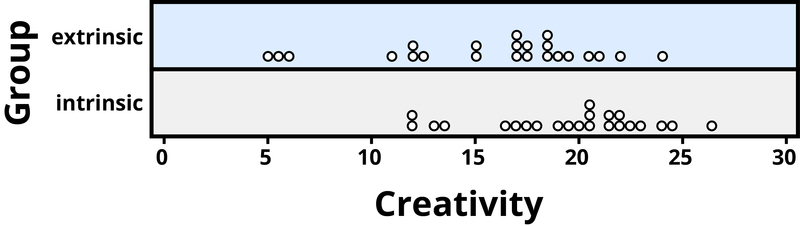
Example 4: A psychology study investigated whether people tend to display more creativity when they are thinking about intrinsic or extrinsic motivations (Ramsey & Schafer, 2002, based on a study by Amabile, 1985). The subjects were 47 people with extensive experience with creative writing. Subjects began by answering survey questions about either intrinsic motivations for writing (such as the pleasure of self-expression) or extrinsic motivations (such as public recognition). Then all subjects were instructed to write a haiku, and those poems were evaluated for creativity by a panel of judges. The researchers conjectured beforehand that subjects who were thinking about intrinsic motivations would display more creativity than subjects who were thinking about extrinsic motivations. The creativity scores from the 47 subjects in this study are displayed in Figure 2, where higher scores indicate more creativity.

예 4: 한 심리학 연구에서는 사람들이 내재적 동기 또는 외재적 동기에 대해 생각할 때 더 많은 창의성을 발휘하는 경향이 있는지에 대해 조사했습니다(Ramsey & Schafer, 2002, Amabile, 1985의 연구를 기반으로 함). 실험 대상은 창의적 글쓰기에 대한 광범위한 경험을 가진 47명이었습니다. 피험자들은 글쓰기의 내재적 동기(예: 자기 표현의 즐거움) 또는 외재적 동기(예: 대중의 인정)에 대한 설문조사 질문에 답하는 것으로 시작하였습니다. 그런 다음 모든 피험자에게 하이쿠를 쓰도록 지시하고 심사위원단의 평가를 통해 창의성을 평가했습니다. 연구진은 내재적 동기에 대해 생각한 피험자가 외재적 동기에 대해 생각한 피험자보다 창의성을 더 많이 발휘할 것이라고 미리 추측했습니다. 이 연구에 참여한 47명의 피험자의 창의성 점수는 그림 2에 표시되어 있으며, 점수가 높을수록 창의성이 높음을 나타냅니다.

Translated with DeepL

In this example, the key question is whether the type of motivation affects creativity scores. In particular, do subjects who were asked about intrinsic motivations tend to have higher creativity scores than subjects who were asked about extrinsic motivations?

이 예에서 핵심 질문은 동기의 유형이 창의성 점수에 영향을 미치는지 여부입니다. 특히 내재적 동기에 대해 질문받은 피험자가 외재적 동기에 대해 질문받은 피험자보다 창의성 점수가 더 높은 경향이 있을까이다.

Figure 2 reveals that both motivation groups saw considerable variability in creativity scores, and these scores have considerable overlap between the groups. In other words, it’s certainly not always the case that those with extrinsic motivations have higher creativity than those with intrinsic motivations, but there may still be a statistical tendency in this direction. (Psychologist Keith Stanovich (2013) refers to people’s difficulties with thinking about such probabilistic tendencies as “the Achilles heel of human cognition.”)

그림 2를 보면 두 동기 부여 그룹 모두 창의성 점수에서 상당한 변동성을 보였으며, 이러한 점수는 그룹 간에 상당히 겹치는 부분이 있음을 알 수 있습니다. 즉, 외재적 동기를 가진 사람이 내재적 동기를 가진 사람보다 항상 창의성이 높은 것은 아니지만, 통계적으로 이러한 방향으로의 경향이 있을 수 있습니다. (심리학자 키스 스타노비치(2013)는 사람들이 이러한 확률적 경향에 대해 생각하는 데 어려움을 겪는 것을 "인간 인지의 아킬레스건"이라고 표현한 바 있습니다.)

The mean creativity score is 19.88 for the intrinsic group, compared to 15.74 for the extrinsic group, which supports the researchers’ conjecture. Yet comparing only the means of the two groups fails to consider the variability of creativity scores in the groups. We can measure variability with statistics using, for instance, the standard deviation: 5.25 for the extrinsic group and 4.40 for the intrinsic group. The standard deviations tell us that most of the creativity scores are within about 5 points of the mean score in each group. We see that the mean score for the intrinsic group lies within one standard deviation of the mean score for extrinsic group. So, although there is a tendency for the creativity scores to be higher in the intrinsic group, on average, the difference is not extremely large.

내재적 그룹의 평균 창의성 점수는 19.88점인 반면 외재적 그룹의 평균 창의성 점수는 15.74점으로 연구진의 추측을 뒷받침합니다. 하지만 두 그룹의 평균만 비교하면 두 그룹의 창의성 점수의 가변성을 고려하지 못합니다. 예를 들어 표준 편차를 사용하여 통계로 가변성을 측정할 수 있습니다: 외재적 그룹의 경우 5.25, 내재적 그룹의 경우 4.40입니다. 표준 편차를 통해 대부분의 창의성 점수가 각 그룹의 평균 점수에서 약 5점 이내에 있음을 알 수 있습니다. 내재적 그룹의 평균 점수는 외재적 그룹의 평균 점수의 1표준편차 내에 있음을 알 수 있습니다. 따라서 내재적 그룹의 창의성 점수가 더 높은 경향은 있지만 평균적으로 그 차이는 그리 크지 않습니다.

We again want to consider possible explanations for this difference. The study only involved individuals with extensive creative writing experience. Although this limits the population to which we can generalize, it does not explain why the mean creativity score was a bit larger for the intrinsic group than for the extrinsic group. Maybe women tend to receive higher creativity scores? Here is where we need to focus on how the individuals were assigned to the motivation groups. If only women were in the intrinsic motivation group and only men in the extrinsic group, then this would present a problem because we wouldn’t know if the intrinsic group did better because of the different type of motivation or because they were women. However, the researchers guarded against such a problem by randomly assigning the individuals to the motivation groups. Like flipping a coin, each individual was just as likely to be assigned to either type of motivation. Why is this helpful? Because this random assignment tends to balance out all the variables related to creativity we can think of, and even those we don’t think of in advance, between the two groups. So we should have a similar male/female split between the two groups; we should have a similar age distribution between the two groups; we should have a similar distribution of educational background between the two groups; and so on. Random assignment should produce groups that are as similar as possible except for the type of motivation, which presumably eliminates all those other variables as possible explanations for the observed tendency for higher scores in the intrinsic group.

이 차이에 대한 가능한 설명을 다시 한 번 생각해보고자 합니다. 이 연구는 창의적인 글쓰기 경험이 풍부한 개인만을 대상으로 했습니다. 이는 일반화할 수 있는 모집단을 제한하지만, 내재적 그룹의 평균 창의성 점수가 외재적 그룹보다 약간 더 높은 이유를 설명하지는 못합니다. 여성이 더 높은 창의성 점수를 받는 경향이 있을까요? 여기서 우리는 개인이 동기 부여 그룹에 어떻게 배정되었는지에 초점을 맞춰야 합니다. 내재적 동기 부여 그룹에는 여성만, 외재적 동기 부여 그룹에는 남성만 배정했다면, 내재적 동기 부여 그룹이 다른 유형의 동기 부여로 인해 더 나은 성과를 냈는지 아니면 여성이기 때문에 더 나은 성과를 냈는지 알 수 없기 때문에 문제가 될 수 있습니다. 그러나 연구진은 개인을 무작위로 동기 부여 그룹에 배정하여 이러한 문제를 방지했습니다. 동전 던지기와 마찬가지로 각 개인은 두 가지 동기 유형에 배정될 확률이 똑같았습니다. 이것이 왜 도움이 될까요? 이러한 무작위 배정은 우리가 생각할 수 있는 창의성과 관련된 모든 변수, 심지어 우리가 미리 생각하지 못한 변수까지 두 그룹 간에 균형을 맞추는 경향이 있기 때문입니다. 따라서 두 그룹 간의 남녀 비율이 비슷해야 하고, 두 그룹 간의 연령 분포가 비슷해야 하며, 두 그룹 간의 학력 분포가 비슷해야 합니다. 무작위 할당은 동기 유형을 제외하고 가능한 한 유사한 그룹을 생성해야 하며, 이는 아마도 내재적 그룹에서 관찰된 높은 점수 경향에 대한 가능한 설명으로 다른 모든 변수를 제거할 것입니다.

But does this always work? No, so by “luck of the draw” the groups may be a little different prior to answering the motivation survey. So then the question is, is it possible that an unlucky random assignment is responsible for the observed difference in creativity scores between the groups? In other words, suppose each individual’s poem was going to get the same creativity score no matter which group they were assigned to, that the type of motivation in no way impacted their score. Then how often would the random-assignment process alone lead to a difference in mean creativity scores as large (or larger) than 19.88 – 15.74 = 4.14 points?

하지만 이것이 항상 효과가 있을까요? 아니요, 동기 부여 설문조사에 응답하기 전에 "추첨의 운"에 따라 그룹이 약간 다를 수 있습니다. 그렇다면 운이 좋지 않은 무작위 배정이 그룹 간 창의성 점수 차이의 원인이 될 수 있을까요? 다시 말해, 각 개인의 시가 어느 그룹에 배정되든 동일한 창의성 점수를 받았고 동기 유형이 점수에 전혀 영향을 미치지 않았다고 가정해 보겠습니다. 그렇다면 무작위 배정 과정만으로 평균 창의성 점수의 차이가 19.88 - 15.74 = 4.14점보다 크거나 더 큰 경우가 얼마나 될까요?

We again want to apply to a probability model to approximate a p-value, but this time the model will be a bit different. Think of writing everyone’s creativity scores on an index card, shuffling up the index cards, and then dealing out 23 to the extrinsic motivation group and 24 to the intrinsic motivation group, and finding the difference in the group means. We (better yet, the computer) can repeat this process over and over to see how often, when the scores don’t change, random assignment leads to a difference in means at least as large as 4.41. Figure 3 shows the results from 1,000 such hypothetical random assignments for these scores.

다시 확률 모델에 적용하여 p값을 근사화하려고 하지만 이번에는 모델이 약간 달라집니다. 모든 사람의 창의성 점수를 색인 카드에 적고 색인 카드를 섞은 다음 외적 동기 부여 그룹에는 23개를, 내적 동기 부여 그룹에는 24개를 나눠서 그룹 간 평균의 차이를 구한다고 생각해 보세요. 이 과정을 계속해서 반복하여 점수가 변하지 않을 때 무작위 할당이 평균의 차이를 최소 4.41만큼 크게 만드는 빈도를 확인할 수 있습니다. 그림 3은 이러한 점수에 대해 이러한 가상의 무작위 할당을 1,000회 수행한 결과를 보여줍니다.

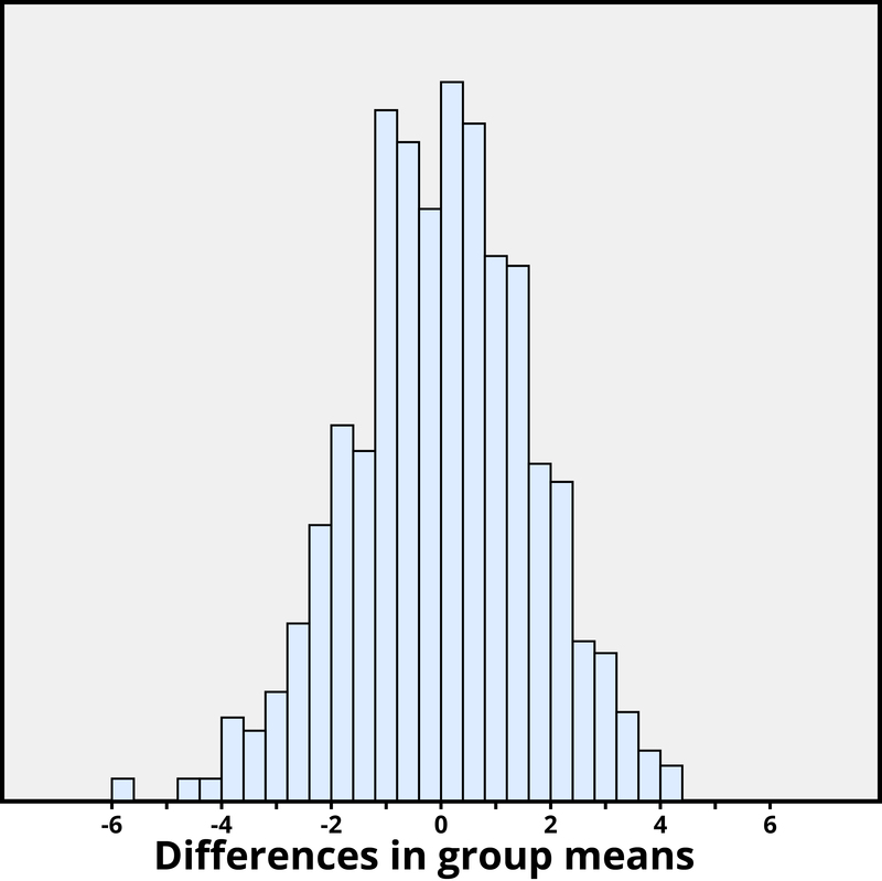
Only 2 of the 1,000 simulated random assignments produced a difference in group means of 4.41 or larger. In other words, the approximate p-value is 2/1000 = 0.002. This small p-value indicates that it would be very surprising for the random assignment process alone to produce such a large difference in group means. Therefore, as with Example 2, we have strong evidence that focusing on intrinsic motivations tends to increase creativity scores, as compared to thinking about extrinsic motivations.

시뮬레이션된 1,000건의 무작위 배정 중 단 2건만이 그룹 평균에 4.41 이상의 차이가 발생했습니다. 즉, 대략적인 p-값은 2/1000 = 0.002입니다. 이 작은 p값은 무작위 할당 프로세스만으로는 그룹 평균에 이렇게 큰 차이가 발생하는 것이 매우 놀랍다는 것을 나타냅니다. 따라서 예 2와 마찬가지로 내재적 동기에 초점을 맞추는 것이 외재적 동기에 대해 생각하는 것보다 창의성 점수를 높이는 경향이 있다는 강력한 증거가 있습니다.

Notice that the previous statement implies a cause-and-effect relationship between motivation and creativity score; is such a strong conclusion justified? Yes, because of the random assignment used in the study. That should have balanced out any other variables between the two groups, so now that the small p-value convinces us that the higher mean in the intrinsic group wasn’t just a coincidence, the only reasonable explanation left is the difference in the type of motivation. Can we generalize this conclusion to everyone? Not necessarily—we could cautiously generalize this conclusion to individuals with extensive experience in creative writing similar the individuals in this study, but we would still want to know more about how these individuals were selected to participate.

앞의 문장은 동기 부여와 창의성 점수 사이의 인과 관계를 암시하고 있는데, 이러한 강력한 결론이 정당한가요? 네, 연구에 사용된 무작위 배정 방식 때문입니다. 따라서 두 그룹 간의 다른 변수가 균형을 이루었을 것이므로, 작은 p값을 통해 내재적 그룹의 평균이 더 높은 것이 우연이 아니라는 것을 확신할 수 있으므로 남은 유일한 합리적인 설명은 동기 유형의 차이뿐입니다. 이 결론을 모든 사람에게 일반화할 수 있을까요? 반드시 그렇지는 않습니다. 이 연구에 참여한 개인과 유사한 창의적 글쓰기 경험이 풍부한 개인에게 이 결론을 조심스럽게 일반화할 수는 있지만, 이러한 개인이 어떻게 참여하도록 선택되었는지에 대해 더 자세히 알고 싶을 것입니다.

결론

Statistical thinking involves the careful design of a study to collect meaningful data to answer a focused research question, detailed analysis of patterns in the data, and drawing conclusions that go beyond the observed data. Random sampling is paramount to generalizing results from our sample to a larger population, and random assignment is key to drawing cause-and-effect conclusions. With both kinds of randomness, probability models help us assess how much random variation we can expect in our results, in order to determine whether our results could happen by chance alone and to estimate a margin of error.

통계적 사고에는 집중된 연구 질문에 답하기 위해 의미 있는 데이터를 수집하고, 데이터의 패턴을 자세히 분석하며, 관찰된 데이터를 뛰어넘는 결론을 도출하기 위한 신중한 연구 설계가 포함됩니다. 무작위 표본 추출은 표본의 결과를 더 큰 집단으로 일반화하기 위해 가장 중요하며, 무작위 할당은 인과관계 결론을 도출하는 데 핵심적인 역할을 합니다. 두 가지 종류의 무작위성을 모두 갖춘 확률 모델은 결과에서 예상할 수 있는 무작위 변동의 정도를 평가하여 결과가 우연에 의해서만 발생할 수 있는지 여부를 판단하고 오차 범위를 추정하는 데 도움이 됩니다.

So where does this leave us with regard to the coffee study mentioned at the beginning of this module? We can answer many of the questions:

• This was a 14-year study conducted by researchers at the National Cancer Institute.
• The results were published in the June issue of the New England Journal of Medicine, a respected, peer-reviewed journal.
• The study reviewed coffee habits of more than 402,000 people ages 50 to 71 from six states and two metropolitan areas. Those with cancer, heart disease, and stroke were excluded at the start of the study. Coffee consumption was assessed once at the start of the study.
• About 52,000 people died during the course of the study.
• People who drank between two and five cups of coffee daily showed a lower risk as well, but the amount of reduction increased for those drinking six or more cups.
• The sample sizes were fairly large and so the p-values are quite small, even though percent reduction in risk was not extremely large (dropping from a 12% chance to about 10%–11%).
• Whether coffee was caffeinated or decaffeinated did not appear to affect the results.
• This was an observational study, so no cause-and-effect conclusions can be drawn between coffee drinking and increased longevity, contrary to the impression conveyed by many news headlines about this study. In particular, it’s possible that those with chronic diseases don’t tend to drink coffee.
• 이 연구는 국립암연구소의 연구원들이 14년에 걸쳐 수행한 연구입니다.
• 이 연구 결과는 권위 있는 동료 심사 저널인 뉴잉글랜드 의학 저널 6월호에 게재되었습니다.
• 이 연구는 6개 주와 2개 대도시에서 50세에서 71세 사이의 402,000명 이상의 커피 습관을 검토했습니다. 연구 시작 시 암, 심장병, 뇌졸중이 있는 사람은 제외되었습니다. 커피 소비량은 연구 시작 시점에 한 번 평가했습니다.
• 연구 기간 동안 약 52,000명이 사망했습니다.
• 매일 2~5잔의 커피를 마시는 사람들도 위험도가 낮았지만, 6잔 이상 마시는 사람들은 위험도 감소폭이 증가했습니다.
• 표본 크기가 상당히 커서 위험 감소율이 매우 크지는 않았지만(12% 확률에서 약 10~11%로 감소) p값은 상당히 작았습니다.
• 커피에 카페인이 들어 있는지, 카페인이 없는지는 결과에 영향을 미치지 않는 것으로 나타났습니다.
• 이 연구는 관찰 연구이므로 이 연구에 대한 많은 뉴스 헤드라인이 전하는 인상과는 달리 커피 음용과 수명 증가 사이에 인과 관계를 결론 내릴 수는 없습니다. 특히 만성 질환이 있는 사람은 커피를 마시지 않는 경향이 있을 수 있습니다.

This study needs to be reviewed in the larger context of similar studies and consistency of results across studies, with the constant caution that this was not a randomized experiment. Whereas a statistical analysis can still “adjust” for other potential confounding variables, we are not yet convinced that researchers have identified them all or completely isolated why this decrease in death risk is evident. Researchers can now take the findings of this study and develop more focused studies that address new questions.

이 연구는 무작위 실험이 아니라는 점을 항상 염두에 두고 유사한 연구와 연구 간 결과의 일관성이라는 더 큰 맥락에서 검토될 필요가 있습니다. 통계 분석을 통해 다른 잠재적 교란 변수를 '조정'할 수는 있지만, 아직 연구자들이 이러한 변수를 모두 파악했거나 사망 위험 감소의 원인을 완전히 밝혀냈다고 확신할 수는 없습니다. 이제 연구자들은 이번 연구 결과를 바탕으로 새로운 질문에 답하는 보다 집중적인 연구를 개발할 수 있습니다.

References

- Amabile, T. (1985). Motivation and creativity: Effects of motivational orientation on creative writers. Journal of Personality and Social Psychology, 48(2), 393–399.
- Freedman, N. D., Park, Y., Abnet, C. C., Hollenbeck, A. R., & Sinha, R. (2012). Association of coffee drinking with total and cause-specific mortality. New England Journal of Medicine, 366, 1891–1904.
- Hamlin, J. K., Wynn, K., & Bloom, P. (2007). Social evaluation by preverbal infants. Nature, 452(22), 557–560.
- Ramsey, F., & Schafer, D. (2002). The statistical sleuth: A course in methods of data analysis. Belmont, CA: Duxbury.
- Short, T., Moriarty, H., & Cooley, M. E. (1995). Readability of educational materials for patients with cancer. Journal of Statistics Education, 3(2).
- Stanovich, K. (2013). How to think straight about psychology (10th ed.). Upper Saddle River, NJ: Pearson.
Authors
Beth ChanceBeth Chance is Professor of Statistics at Cal Poly - San Luis Obispo. She is a Fellow of the American Statistical Association, the inaugural winner of the Waller Education Award for excellence and innovation in teaching undergraduate statistics, and a 2011 MERLOT Classics Award for technology tools development.
Allan RossmanAllan Rossman, Professor of Statistics at Cal Poly – San Luis Obispo, has written curricular materials and conducted many faculty development workshops related to undergraduate statistics education. He is a Fellow of the American Statistical Association and a recipient of the Mathematical Association of America’s Haimo Award for Distinguished Teaching.
Creative Commons License
Statistical Thinking by Beth Chance and Allan Rossman is licensed under a Creative Commons Attribution-NonCommercial-ShareAlike 4.0 International License. Permissions beyond the scope of this license may be available in our Licensing Agreement.